Upload H5 File From Google Drive Into Google Colab
![]()
Analysis examples#
In this notebook we'll show examples of how you might use the predictions exported from SLEAP. We'll piece of work with an Analysis HDF5 file (rather than the .slp predictions file). This HDF5 file tin can exist exported from SLEAP.
Nosotros suggest building your mail-SLEAP analysis pipeline around these HDF5 files rather than trying to work straight with the .slp files used by SLEAP.
Note: You can work with these HDF5 directly in Python (every bit nosotros'll do here) or MATLAB without having SLEAP itself installed.
Case analysis information#
Let'due south start by download a sample HDF5. These predictions were created with models trained on our sample Drosophila melanogaster courtship dataset. Using these models we tin inference on a video clip with 3000 frames. The video clip, resulting predictions, and exported HDF5 are all available here.
We'll just download the predictions.analysis.h5 file:
!wget -O predictions.analysis.h5 https://github.com/murthylab/sleap/raw/main/docs/notebooks/analysis_example/predictions.analysis.h5 --2021-01-04 03:24:05-- https://github.com/murthylab/sleap/raw/master/docs/notebooks/analysis_example/predictions.analysis.h5 Resolving github.com (github.com)... 140.82.113.iv Connecting to github.com (github.com)|140.82.113.4|:443... connected. HTTP request sent, awaiting response... 302 Establish Location: https://raw.githubusercontent.com/murthylab/sleap/primary/docs/notebooks/analysis_example/predictions.analysis.h5 [following] --2021-01-04 03:24:05-- https://raw.githubusercontent.com/murthylab/sleap/tree/main/docs/notebooks/analysis_example/predictions.analysis.h5 Resolving raw.githubusercontent.com (raw.githubusercontent.com)... 151.101.0.133, 151.101.64.133, 151.101.128.133, ... Connecting to raw.githubusercontent.com (raw.githubusercontent.com)|151.101.0.133|:443... connected. HTTP asking sent, awaiting response... 200 OK Length: 551501 (539K) [awarding/octet-stream] Saving to: 'predictions.analysis.h5' predictions.analysi 100%[===================>] 538.58K --.-KB/s in 0.05s 2021-01-04 03:24:05 (ten.5 MB/south) - 'predictions.assay.h5' saved [551501/551501]
We can set the path and filename to the analysis HDF5. In our case, this is just predictions.analysis.h5 . If y'all're running analysis code on your local computer this will exist the full path and filename of your HDF5. If you're running assay code on Colab, and then yous'll probably re-create files to Colab via Google Drive and should use the path to your file there.
filename = "predictions.analysis.h5"
Loading the data#
We use the h5py packet to load data from the HDF5. This is already installed in Colab. If your running analysis lawmaking on your local machine and have SLEAP installed, then h5py and other packages we use are already installed in your SLEAP conda environment. Otherwise, you may need to use conda or pip to install h5py likewise as numpy , scipy , matplotlib , seaborn , and any other packages y'all want use in your analysis lawmaking.
Let's load the file and take a peek.
import h5py import numpy as np with h5py . File ( filename , "r" ) as f : dset_names = list ( f . keys ()) locations = f [ "tracks" ][:] . T node_names = [ n . decode () for northward in f [ "node_names" ][:]] impress ( "===filename===" ) print ( filename ) print () print ( "===HDF5 datasets===" ) impress ( dset_names ) print () print ( "===locations data shape===" ) print ( locations . shape ) print () print ( "===nodes===" ) for i , name in enumerate ( node_names ): print ( f " { i } : { name } " ) print ()
===filename=== predictions.assay.h5 ===HDF5 datasets=== ['node_names', 'track_names', 'track_occupancy', 'tracks'] ===locations data shape=== (3000, xiii, two, 2) ===nodes=== 0: head 1: thorax ii: abdomen 3: wingL iv: wingR v: forelegL4 6: forelegR4 7: midlegL4 eight: midlegR4 nine: hindlegL4 10: hindlegR4 11: eyeL 12: eyeR
In our example file, the shape of the locations matrix (the tracks dataset) is (3000, xiii, two, two) afterwards it is transposed (with the .T ). We transpose the information when loading it in Python; no transpose is needed when using MATLAB. This is because Python and MATLAB wait matrices to exist stored differently.
Hither's what each dimension of the matrix ways:
-
3000: the number of frames;
-
13: the number of nodes in the skeleton (we've also loaded and displayed the
node_namesdataset with the names of these 13 nodes); -
2: for the x and y coordinates;
-
2: the number of distinct animal identities which were found (we accept ii flies in the video clip and they were tracked perfectly, and then we ended up with exactly 2 track, simply there may be more tracks than animals if tracking didn't work as well).
We tin get these counts from the shape of the matrix, like so:
frame_count , node_count , _ , instance_count = locations . shape impress ( "frame count:" , frame_count ) impress ( "node count:" , node_count ) print ( "case count:" , instance_count )
frame count: 3000 node count: xiii case count: ii
Now that we've loaded the data, permit's see some dissimilar things nosotros can do with it…
Fill missing values#
from scipy.interpolate import interp1d def fill_missing ( Y , kind = "linear" ): """Fills missing values independently along each dimension later the first.""" # Store initial shape. initial_shape = Y . shape # Flatten after first dim. Y = Y . reshape (( initial_shape [ 0 ], - ane )) # Interpolate along each slice. for i in range ( Y . shape [ - 1 ]): y = Y [:, i ] # Build interpolant. 10 = np . flatnonzero ( ~ np . isnan ( y )) f = interp1d ( x , y [ x ], kind = kind , fill_value = np . nan , bounds_error = False ) # Fill missing xq = np . flatnonzero ( np . isnan ( y )) y [ xq ] = f ( xq ) # Fill leading or trailing NaNs with the nearest not-NaN values mask = np . isnan ( y ) y [ mask ] = np . interp ( np . flatnonzero ( mask ), np . flatnonzero ( ~ mask ), y [ ~ mask ]) # Save slice Y [:, i ] = y # Restore to initial shape. Y = Y . reshape ( initial_shape ) return Y
locations = fill_missing ( locations )
Visualize thorax movement across video#
HEAD_INDEX = 0 THORAX_INDEX = 1 ABDO_INDEX = ii head_loc = locations [:, HEAD_INDEX , :, :] thorax_loc = locations [:, THORAX_INDEX , :, :] abdo_loc = locations [:, ABDO_INDEX , :, :]
import seaborn as sns import matplotlib as mpl import matplotlib.pyplot as plt
sns . fix ( 'notebook' , 'ticks' , font_scale = 1.2 ) mpl . rcParams [ 'figure.figsize' ] = [ 15 , six ]
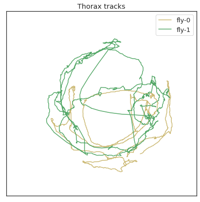
plt . figure () plt . plot ( thorax_loc [:, 0 , 0 ], 'y' , characterization = 'wing-0' ) plt . plot ( thorax_loc [:, 0 , 1 ], 'g' , label = 'fly-1' ) plt . plot ( - 1 * thorax_loc [:, 1 , 0 ], 'y' ) plt . plot ( - 1 * thorax_loc [:, 1 , 1 ], 'yard' ) plt . legend ( loc = "center right" ) plt . title ( 'Thorax locations' ) plt . figure ( figsize = ( seven , 7 )) plt . plot ( thorax_loc [:, 0 , 0 ], thorax_loc [:, 1 , 0 ], 'y' , label = 'fly-0' ) plt . plot ( thorax_loc [:, 0 , 1 ], thorax_loc [:, i , one ], 'one thousand' , label = 'wing-ane' ) plt . legend () plt . xlim ( 0 , 1024 ) plt . xticks ([]) plt . ylim ( 0 , 1024 ) plt . yticks ([]) plt . title ( 'Thorax tracks' )
Text(0.5, ane.0, 'Thorax tracks') 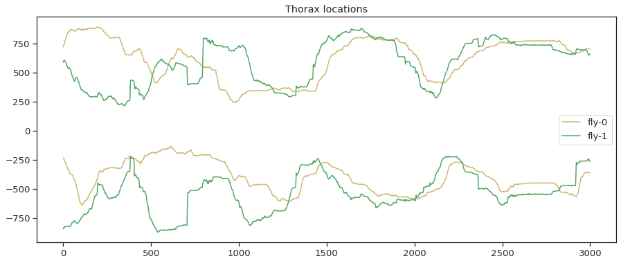
More avant-garde visualizations#
For some additional assay, we'll first smoothen and differentiate the data with a Savitzky-Golay filter to extract velocities of each joint.
from scipy.indicate import savgol_filter def smooth_diff ( node_loc , win = 25 , poly = 3 ): """ node_loc is a [frames, two] array win defines the window to smoothen over poly defines the society of the polynomial to fit with """ node_loc_vel = np . zeros_like ( node_loc ) for c in range ( node_loc . shape [ - 1 ]): node_loc_vel [:, c ] = savgol_filter ( node_loc [:, c ], win , poly , deriv = 1 ) node_vel = np . linalg . norm ( node_loc_vel , axis = 1 ) return node_vel
There are two flies. Let's become results for each separately.
thx_vel_fly0 = smooth_diff ( thorax_loc [:, :, 0 ]) thx_vel_fly1 = smooth_diff ( thorax_loc [:, :, i ])
Visualizing thorax x-y dynamics and velocity for fly 0#
fig = plt . figure ( figsize = ( 15 , 7 )) ax1 = fig . add_subplot ( 211 ) ax1 . plot ( thorax_loc [:, 0 , 0 ], 'thou' , label = 'x' ) ax1 . plot ( - 1 * thorax_loc [:, 1 , 0 ], 'k' , label = 'y' ) ax1 . fable () ax1 . set_xticks ([]) ax1 . set_title ( 'Thorax' ) ax2 = fig . add_subplot ( 212 , sharex = ax1 ) ax2 . imshow ( thx_vel_fly0 [:, np . newaxis ] . T , aspect = 'auto' , vmin = 0 , vmax = 10 ) ax2 . set_yticks ([]) ax2 . set_title ( 'Velocity' )
Text(0.v, ane.0, 'Velocity') 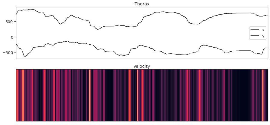
Visualize thorax colored by magnitude of wing speed#
fig = plt . effigy ( figsize = ( 15 , half dozen )) ax1 = fig . add_subplot ( 121 ) ax1 . plot ( thorax_loc [:, 0 , 0 ], thorax_loc [:, 1 , 0 ], 'thousand' ) ax1 . set_xlim ( 0 , 1024 ) ax1 . set_xticks ([]) ax1 . set_ylim ( 0 , 1024 ) ax1 . set_yticks ([]) ax1 . set_title ( 'Thorax tracks' ) kp = thx_vel_fly0 # use thx_vel_fly1 for other fly vmin = 0 vmax = 10 ax2 = fig . add_subplot ( 122 ) ax2 . besprinkle ( thorax_loc [:, 0 , 0 ], thorax_loc [:, one , 0 ], c = kp , southward = 4 , vmin = vmin , vmax = vmax ) ax2 . set_xlim ( 0 , 1024 ) ax2 . set_xticks ([]) ax2 . set_ylim ( 0 , 1024 ) ax2 . set_yticks ([]) ax2 . set_title ( 'Thorax tracks colored by magnitude of wing speed' )
Text(0.5, 1.0, 'Thorax tracks colored by magnitude of fly speed') 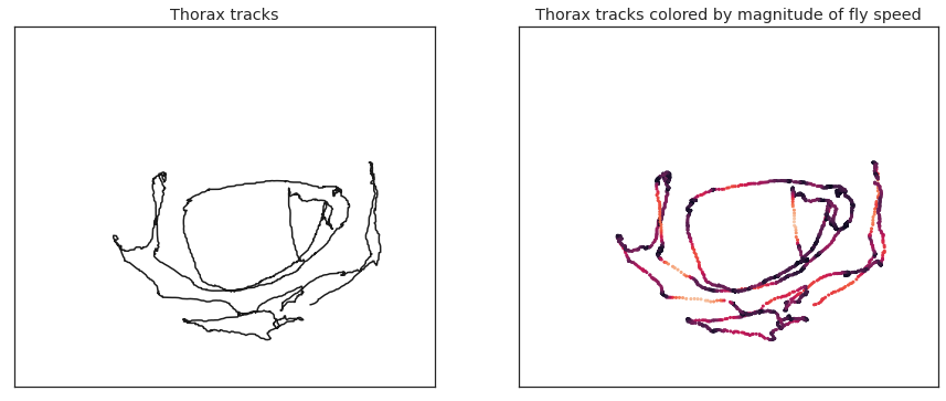
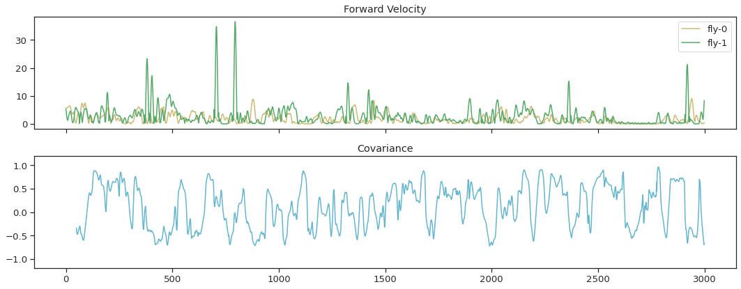
Observe covariance in thorax velocities betwixt fly-0 and fly-ane#
import pandas as pd def corr_roll ( datax , datay , win ): """ datax, datay are the ii timeseries to discover correlations betwixt win sets the number of frames over which the covariance is computed """ s1 = pd . Series ( datax ) s2 = pd . Series ( datay ) render np . array ( s2 . rolling ( win ) . corr ( s1 ))
win = 50 cov_vel = corr_roll ( thx_vel_fly0 , thx_vel_fly1 , win ) fig , ax = plt . subplots ( ii , 1 , sharex = True , figsize = ( xv , 6 )) ax [ 0 ] . plot ( thx_vel_fly0 , 'y' , label = 'fly-0' ) ax [ 0 ] . plot ( thx_vel_fly1 , 'g' , label = 'fly-i' ) ax [ 0 ] . legend () ax [ 0 ] . set_title ( 'Forrard Velocity' ) ax [ 1 ] . plot ( cov_vel , 'c' , markersize = one ) ax [ 1 ] . set_ylim ( - 1.2 , 1.2 ) ax [ one ] . set_title ( 'Covariance' ) fig . tight_layout ()
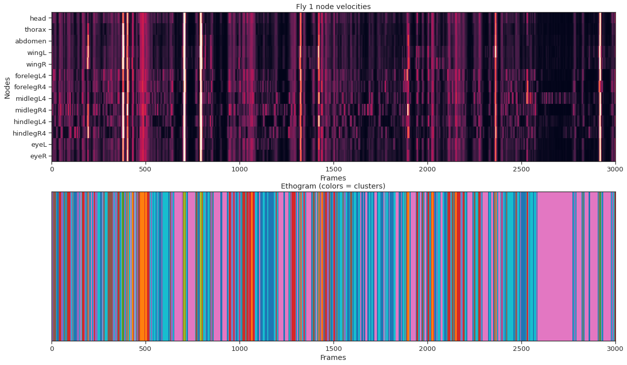
Clustering#
For an example of clustering the data, we'll
-
extract articulation velocities for each articulation,
-
run uncomplicated k-ways on the velocities from each frame.
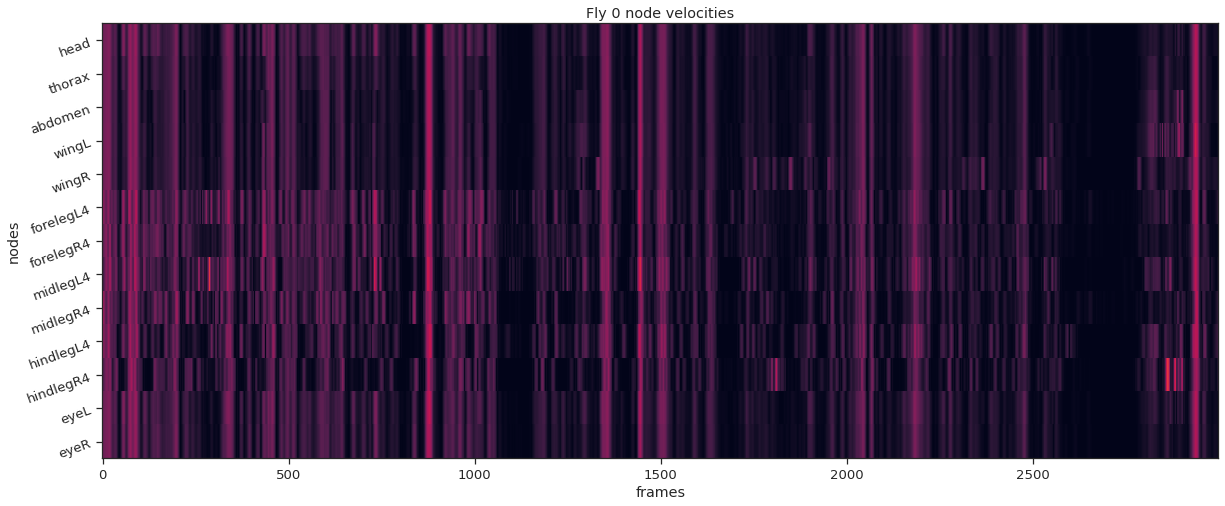
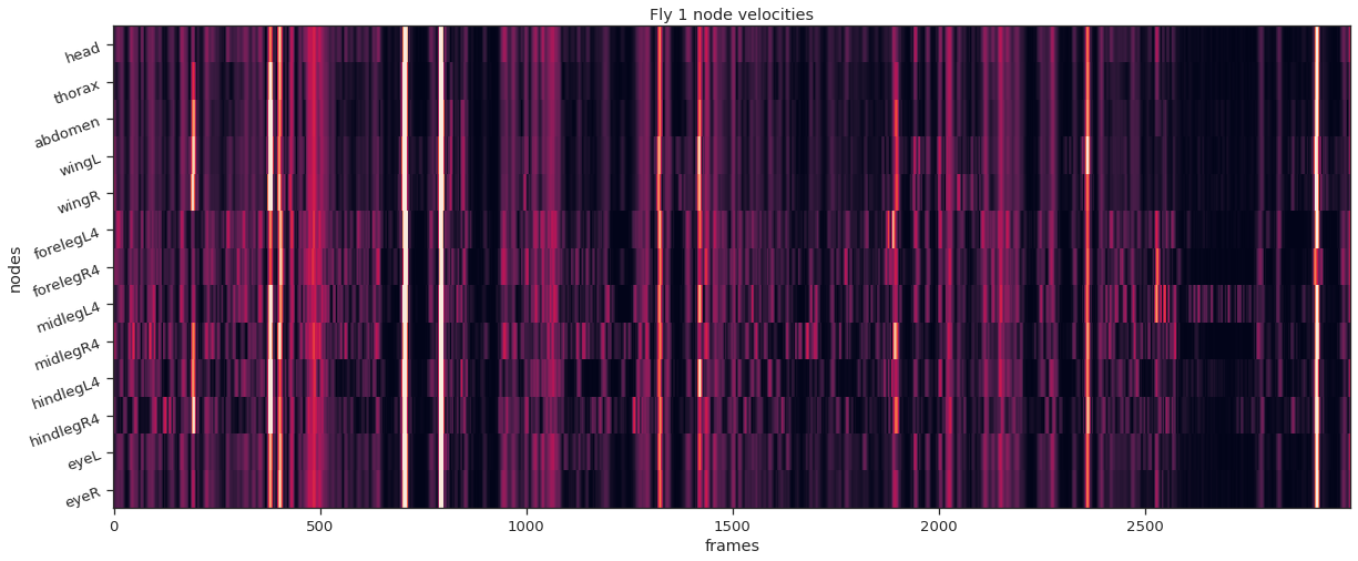
def instance_node_velocities ( instance_idx ): fly_node_locations = locations [:, :, :, instance_idx ] fly_node_velocities = np . zeros (( frame_count , node_count )) for n in range ( 0 , node_count ): fly_node_velocities [:, n ] = smooth_diff ( fly_node_locations [:, n , :]) return fly_node_velocities
def plot_instance_node_velocities ( instance_idx , node_velocities ): plt . effigy ( figsize = ( 20 , 8 )) plt . imshow ( node_velocities . T , attribute = 'automobile' , vmin = 0 , vmax = 20 , interpolation = "nearest" ) plt . xlabel ( 'frames' ) plt . ylabel ( 'nodes' ) plt . yticks ( np . arange ( node_count ), node_names , rotation = 20 ); plt . title ( f 'Fly { instance_idx } node velocities' )
fly_ID = 0 fly_node_velocities = instance_node_velocities ( fly_ID ) plot_instance_node_velocities ( fly_ID , fly_node_velocities )
fly_ID = i fly_node_velocities = instance_node_velocities ( fly_ID ) plot_instance_node_velocities ( fly_ID , fly_node_velocities )
from sklearn.cluster import KMeans
nstates = 10 km = KMeans ( n_clusters = nstates ) labels = km . fit_predict ( fly_node_velocities )
fig = plt . figure ( figsize = ( 20 , 12 )) ax1 = fig . add_subplot ( 211 ) ax1 . imshow ( fly_node_velocities . T , aspect = "auto" , vmin = 0 , vmax = 20 , interpolation = "nearest" ) ax1 . set_xlabel ( "Frames" ) ax1 . set_ylabel ( "Nodes" ) ax1 . set_yticks ( np . arange ( node_count )) ax1 . set_yticklabels ( node_names ); ax1 . set_title ( f "Fly { fly_ID } node velocities" ) ax1 . set_xlim ( 0 , frame_count ) ax2 = fig . add_subplot ( 212 , sharex = ax1 ) ax2 . imshow ( labels [ None , :], aspect = "auto" , cmap = "tab10" , interpolation = "nearest" ) ax2 . set_xlabel ( "Frames" ) ax2 . set_yticks ([]) ax2 . set_title ( "Ethogram (colors = clusters)" );
Source: https://sleap.ai/notebooks/Analysis_examples.html
0 Response to "Upload H5 File From Google Drive Into Google Colab"
Post a Comment